ランベルトのW関数

ランベルトのW函数（ランベルトのWかんすう、英: Lambert W function）あるいはオメガ函数 (ω function)、対数積（product logarithm; 乗積対数）は、函数 f(z) = ze^z の逆関係の分枝として得られる函数 W の総称である。ここで、e^z は指数函数、z は任意の複素数とする。すなわち、W は z = f⁻¹(ze^z) = W(ze^z) を満たす。

上記の方程式で、z' = ze^z と置きかえれば、任意の複素数 z' に対する W 函数（一般には W 関係）の定義方程式

${\displaystyle z'=W(z')e^{W(z')}}$

を得る。

函数 ƒ は単射ではないから、関係 W は（0 を除いて）多価である。仮に実数値の W に注意を制限するとすれば、複素変数 z は実変数 x に取り換えられ、関係の定義域は区間 x ≥ −1/e に限られ、また開区間 (−1/e, 0) 上で二価の函数になる。さらに制約条件として W ≥ −1 を追加すれば一価函数 W₀(x) が定義されて、W₀(0) = 0 および W₀(−1/e) = −1 を得る。それと同時に、下側の枝は W ≤ −1 であって、W₋₁(x) と書かれる。これは W₋₁(−1/e) = −1 から W₋₁(−0) = −∞ まで単調減少する。

ランベルト W 関係は初等函数では表すことができない^[1]。ランベルト W は組合せ論において有用で、例えば木の数え上げに用いられる。指数函数を含む様々な方程式（例えばプランク分布、ボーズ–アインシュタイン分布、フェルミ–ディラック分布などの最大値）を解くのに用いられ、またy'(t) = ay(t − 1) のような遅延微分方程式（英語版） の解としても生じる。生化学において、また特に酵素動力学において、ミカエリス–メンテン動力学の経時動力学解析に対する閉じた形の解はランベルト W 函数によって記述される。

用語について

ランベルト W-函数はヨハン・ハインリヒ・ランベルトに因んで名づけられた。Digital Library of Mathematical Functions では主枝 W₀ を Wp, 分枝 W₋₁ は Wm と書いている。ここでの表記の規約（つまり W₀, W₋₁）はランベルト W に関する標準的な参考文献Corless et al. (1996)^[2]に従った。

歴史

ランベルトは初め「ランベルトの超越方程式」に関連して1758年に考察した^[3]。これはレオンハルト・オイラーの1783年の we^w の特別な場合を論じた論文^[4]に繋がる。

ランベルト W-函数は、特殊化された応用において、十年程度毎に「再発見」されてきた^[要出典]。1993年には、等電荷に対する量子力学的二重井戸型ディラックデルタ函数モデル（英語版）（物理学における基本問題）の厳密解をランベルト W-函数が与えることが報告されたとき、コーレスら計算機代数システムMapleの開発者たちはライブラリを精査して、この函数が自然界に遍く存在することを発見した^[2][5]。

微分積分学

導函数

陰函数微分法により、W の任意の枝が常微分方程式

${\displaystyle z(1+W){\frac {dW}{dz}}=W\quad (z\neq -1/e)}$

を満たすことが示せる（z = −1/e では W は微分できない）。従って、W の導函数は

${\displaystyle {\frac {dW}{dz}}={\frac {W(z)}{z(1+W(z))}}\quad (z\notin \{0,-1/e\})}$

を満たす。ここで恒等式 e^W(z) = z/W(z) を用いるならば、

${\displaystyle {\frac {dW}{dz}}={\frac {1}{z+e^{W(z)}}}\quad (z\neq -1/e)}$

と書きなおすこともできる。

原始函数

函数 W(x)（およびそれを含む多くの式）は、w = W(x), (x = we^w) と置いた置換積分によって

${\displaystyle {\begin{aligned}\int W(x){\mathit {dx}}&=xW(x)-x+e^{W(x)}+C\\&=x\left(W(x)-1+{\frac {1}{W(x)}}\right)+C.\\\end{aligned}}}$

と積分できる。

したがって、（W(e) = 1 であることも考慮して）等式

${\displaystyle \int _{0}^{e}W(x)\,{\mathit {dx}}=e-1}$

が得られる。

漸近展開

W₀ の 0 を中心とするテイラー級数は、逆に解いて（英語版）

${\displaystyle W_{0}(x)=\sum _{n=1}^{\infty }{\frac {(-n)^{n-1}}{n!}}\ x^{n}=x-x^{2}+{\frac {3}{2}}x^{3}-{\frac {8}{3}}x^{4}+{\frac {125}{24}}x^{5}-\cdots }$

ダランベールの収束判定法によると、収束半径は 1⁄e である。この級数の定める函数は、区間 (−∞, −1/e]に沿って分岐切断（英語版）を入れれば、ガウス平面の全域で定義される正則函数に延長することができる。この正則函数をランベルト W 函数の主値と定める。

x が十分大きければ、W₀ は漸近的に

${\displaystyle {\begin{aligned}W_{0}(x)&=L_{1}-L_{2}+{\frac {L_{2}}{L_{1}}}+{\frac {L_{2}(-2+L_{2})}{2L_{1}^{2}}}\\&\qquad \qquad +{\frac {L_{2}(6-9L_{2}+2L_{2}^{2})}{6L_{1}^{3}}}+{\frac {L_{2}(-12+36L_{2}-22L_{2}^{2}+3L_{2}^{3})}{12L_{1}^{4}}}+\cdots \\[8pt]&=L_{1}-L_{2}+\sum _{\ell =0}^{\infty }\sum _{m=1}^{\infty }{\frac {(-1)^{\ell }\left[{\ell +m \atop \ell +1}\right]}{m!}}L_{1}^{-\ell -m}L_{2}^{m}\\&=\ln(x)-\ln(\ln(x))+o(1)\end{aligned}}}$

と展開される。ただし、L₁ = ln(x), L₂ = ln(ln(x)) であり、[k
n ] は非負の第一種スターリング数である^[6]。

もう一つの、区間 (−∞, −1/e] 上で定義される実函数な枝 W₋₁ は、L₁ = ln(−x), L₂ = ln(−ln(−x)) と書けば、x が十分 0 に近いとき同じ形の漸近展開を持つ。

x ≥ e なるとき、

${\displaystyle \ln(x)-\ln {\bigl (}\ln(x){\bigr )}+{\frac {\ln {\bigl (}\ln(x){\bigr )}}{2\ln(x)}}\leq W_{0}(x)\leq \ln(x)-\ln {\bigl (}\ln(x){\bigr )}+{\frac {e}{e-1}}{\frac {\ln {\bigl (}\ln(x){\bigr )}}{\ln(x)}}}$

という上下の評価が成り立つ^[7]。また もう一つの枝 W₋₁ の評価は u > 0 に対して

${\displaystyle -1-{\sqrt {2u}}-u<W_{-1}(-e^{-u-1})<-1-{\sqrt {2u}}-{\frac {2}{3}}u}$

となる^[8]。

整数冪・複素数冪の展開

W₀ の整数乗もまた 0 において単純なテイラー級数（あるいはローラン級数）展開を持つ。例えば

${\displaystyle W_{0}(x)^{2}=\sum _{n=2}^{\infty }{\frac {-2(-n)^{n-3}}{(n-2)!}}\ x^{n}=x^{2}-2x^{3}+4x^{4}-{\frac {25}{3}}x^{5}+18x^{6}-\cdots .}$

より一般に、ラグランジュの反転公式を用いれば、r ∈ Z に対して

${\displaystyle W_{0}(x)^{r}=\sum _{n=r}^{\infty }{\frac {-r(-n)^{n-r-1}}{(n-r)!}}\ x^{n}}$

となることが示せる（これは一般に、位数 r のローラン級数になっている）。あるいは同じことだが、この式を W₀(x)/x の冪に関するテイラー級数として

${\displaystyle \left({\frac {W_{0}(x)}{x}}\right)^{r}=\exp(-rW_{0}(x))=\sum _{n=0}^{\infty }{\frac {r(n+r)^{n-1}}{n!}}(-x)^{n}}$

と書くことができる。これは任意の r ∈ C と |x| < e⁻¹ に対して成立する。

特殊値

任意の非零代数的数 x に対して W(x) は超越数になる。実際、W(x) が零ならば x も零でなければならず、また W(x) が非零代数的数ならばリンデマン–ワイエルシュトラスの定理により e^W(x) は超越的でなければならず、従ってx = W(x)e^W(x) もまた超越的でなければならない。

${\displaystyle W(-\pi /2)=i\pi /2}$

${\displaystyle W({\ln 4})=\ln 2}$

${\displaystyle W_{0}(-(\ln 2)/2)=-\ln 2}$

${\displaystyle W_{-1}(-(\ln 2)/2)=W_{-1}(-(\ln 4)/4)=-\ln 4}$

${\displaystyle W(-(\ln a)/a)=-\ln a\quad (1/e\leq a\leq e)}$

${\displaystyle W(-1/e)=-1}$

${\displaystyle W(0)=0}$

${\displaystyle W(1)=\Omega ={\frac {1}{\displaystyle \int _{-\infty }^{+\infty }{\frac {dt}{(e^{t}-t)^{2}+\pi ^{2}}}}}-1\approx 0.56714329\dots }$ (オメガ定数)

${\displaystyle W(1)=e^{-W(1)}=-\ln W(1)}$

${\displaystyle W(e)=1}$

${\displaystyle -W(-1)=e^{-W(-1)}=\ln(-{W(-1)})\approx 0.31813\dots \ +1.33723\dots \,i}$

${\displaystyle W'(0)=1}$

等式

いくつかの等式は定義から直ちに得られる:

${\displaystyle {\begin{aligned}W(xe^{x})&=x&(x\geq 0,\,x=-1)\\W_{0}(xe^{x})&=x&(x\geq -1)\\W_{-1}(xe^{x})&=x&(x\leq -1)\end{aligned}}}$

ここで、f(x) = x⋅e^x は単射でないから、W(f(x)) = x は常には成り立たないことに注意すべきである。x < 0 かつ x ≠ -1 なる x を固定して、方程式 x⋅e^x = y⋅e^y は y に関して二つの解を持ち、その一方はもちろん y = x である。もう一方の解は、W₀ の場合 x < -1 に、W₋₁ の場合 x ∈ (-1, 0) にある。これらを踏まえて、次の式を導くことができる。

${\displaystyle W_{0}(xe^{x})=y\quad (x<-1).}$

${\displaystyle W_{-1}(xe^{x})=y\quad (x>-1).}$

${\displaystyle W(x)e^{W(x)}=x.}$

${\displaystyle e^{W(x)}=x/W(x).}$

${\displaystyle W(x)=\ln x-\ln W(x)\quad (x\geq -1/e).}$

${\displaystyle \ln W(x)=\ln x-W(x)\quad (x>0).}$^[9]

${\displaystyle W(nx^{n}/W(x)^{n-1})=nW(x)\quad (n>0,x>0).}$（これは正しく枝を選べば他の n, x に対しても拡張できる）

f(ln(x)) を反転すれば

${\displaystyle W(x\ln x)=\ln x=W(x)+\ln W(x)\quad (x>0)}$

を得る。

オイラーの反復指数函数 h(x) を用いれば

${\displaystyle h(x)=e^{-W(-\ln(x))}={\frac {W(-\ln(x))}{-\ln(x)}}\quad (x\neq 1)}$

を得る。

W を含む有用な積分公式がいくつか存在し、例えば以下のようなものが挙げられる:

分岐切断 (−∞, 1/e] に沿う z を除けば（そのような z では以下の積分が確定しない）、ランベルト W 函数の主枝は、以下の積分

${\displaystyle W(z)={\frac {z}{2\pi }}\int \limits _{-\pi }^{\pi }{\frac {(1-\nu \cot \nu )^{2}+\nu ^{2}}{z+\nu \csc \nu e^{-\nu \cot \nu }}}d\nu ={\frac {z}{\pi }}\int \limits _{0}^{\pi }{\frac {(1-\nu \cot \nu )^{2}+\nu ^{2}}{z+\nu \csc \nu e^{-\nu \cot \nu }}}d\nu }$

によって計算できる^[10]。この二つの積分の値が等しいことは被積分函数の対称性による。

応用

指数関数を含む方程式の多くは、W関数を用いることで解くことができる。主な方針は、未知数を含む項を方程式の左辺（あるいは右辺）に寄せ、W関数で解を表現できる ${\displaystyle xe^{x}}$の形にすることである。例えば、方程式 ${\displaystyle 2^{t}=5t}$ を解くには、両辺に ${\displaystyle -{\frac {\ln 2\cdot 2^{-t}}{5}}}$を掛け、${\displaystyle -{\frac {\ln 2}{5}}=-t\ln 2\cdot e^{-t\ln 2}}$を得る。

ここで、両辺のW関数をとれば、${\displaystyle W\left(-{\frac {\ln 2}{5}}\right)=-t\ln 2}$、即ち ${\displaystyle t=-{\frac {W\left(-{\frac {\ln {2}}{5}}\right)}{\ln {2}}}=0.235\dots ,4.488\dots }$となる。

同様の方法で、x^x = z の解は、

あるいは

となる。

複素数の無限回の累乗

が収束するとき、ランベルトのW関数を用いれば、その極限値を次のように表現できる。

ただし、log(z) は複素対数函数の主値とする。

一般化

通常のランベルト W は x に関する

の形（ただし、a₀, c, r は実定数）の「超越代数」方程式の厳密解 x = r + 1/cW(ce^−cr/a₀) を記述することができる。

ランベルト W 函数の一般化^{[11][12][13][14]}として以下のようなものを挙げることができる:

• 低次元における一般相対論および量子力学（量子重力）（実は、両分野の繋がりは、以前には知られていなかった^[15]）への応用では、式 1 の右辺を今度は x の二次多項式とした

を考える。ここで、この二次多項式の根 r₁, r₂ は相異なる実定数とする。この方程式の解は一つの引数 x を持つ函数だが、r_i や a₀ のような項は解函数のパラメータとして働く。そのような側面で見れば、この一般化は超幾何函数やメイヤーG函数（英語版）を作るのと似たような方式とも思えるが、これらの函数とは異なる「クラス」に属する。r₁ = r₂ のときは、式 2 の両辺は因数分解できて、1 に帰着されるから、解函数も通常の W 函数に還元される。式 2 はディラトン場を支配する方程式を表すから、それにより不等静止質量の場合に対する 1+1-次元（空間一次元・時間一次元）における R=T（英語版）あるいは「直列」(lineal) 二体重力問題の計量や、一次元の不等電荷に対する量子力学的二重井戸型デルタ函数モデル（英語版）の固有エネルギーが導かれる。

• 量子力学的三体問題（英語版）の特別の場合、具体的には（三次元）水素分子イオン^[16]の固有エネルギーの解析解の場合、今度は式 1 の（あるいは式 2 の）右辺を x に関する無限次多項式の比とした

を考える。各 r_i, s_i は実定数、x は固有エネルギーと核間距離 R の函数である。式 3 は、その特別の場合として式 1 および 2 も含めて、遅延微分方程式（英語版）の成す大きなクラスに関係する。

(1)式で表現される標準的な場合においても、原子・分子・光物理学^[17] などの分野>からリーマン仮説^[18]に対するKeiper-Li基準に至るまで、ランベルトのW函数の応用分野についての議論は十分尽くされたとは言えていない。

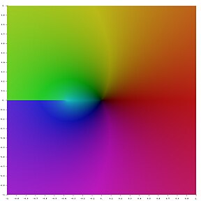
複素平面上のグラフ

• Plots of the Lambert W function on the complex plane
• 
  z = Re(W₀(x + iy))
• 
  z = Im(W₀(x + iy))
• 
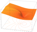  z = |W₀(x + iy)|
• 
  Superimposition of the previous three plots

数値的評価

W 函数はニュートン法を用いて近似することができて、w = W(z)（したがって z = we^w）に対する逐次近似は

${\displaystyle w_{j+1}=w_{j}-{\frac {w_{j}e^{w_{j}}-z}{e^{w_{j}}+w_{j}e^{w_{j}}}}}$

として与えられる。また、ハレー法（英語版） を用いた近似

${\displaystyle w_{j+1}=w_{j}-{\frac {w_{j}e^{w_{j}}-z}{e^{w_{j}}(w_{j}+1)-{\frac {(w_{j}+2)(w_{j}e^{w_{j}}-z)}{2w_{j}+2}}}}}$

を Corless et al. (1996) は W の計算において与えている。

ソフトウェア実装

W 函数の実装は:

• LambertW in Maple,
• lambertw in GP (glambertW in PARI),
• lambertw in MATLAB,^[19]
• lambertw in octave with the 'specfun' package,
• lambert_w in Maxima,^[20]
• ProductLog (with a silent alias LambertW) in Mathematica,^[21]
• lambertw in Python scipy's special function package^[22]
• gsl_sf_lambert_W0 and gsl_sf_lambert_Wm1 functions in special functions section of the GNU Scientific Library - GSL.

などがある。

関連項目

• 重み付きオメガ函数（英語版）
• ランベルトの三項方程式
• ラグランジュの反転定理（英語版）
• 実験数学
• ホルスタイン–ヘーリング法（英語版）
• R=Tモデル（英語版）
• ロスのπ補題（英語版）

脚注

参考文献

• Corless, R.; Gonnet, G.; Hare, D.; Jeffrey, D.; Knuth, Donald (1996). “On the Lambert W function”. Advances in Computational Mathematics (Berlin, New York: Springer-Verlag) 5: 329–359. doi:10.1007/BF02124750. ISSN 1019-7168. http://www.apmaths.uwo.ca/~djeffrey/Offprints/W-adv-cm.pdf 
• Chapeau-Blondeau, F.; Monir, A. (2002). “Evaluation of the Lambert W Function and Application to Generation of Generalized Gaussian Noise With Exponent 1/2”. IEEE Trans. Signal Processing 50 (9). http://www.istia.univ-angers.fr/~chapeau/papers/lambertw.pdf. 
• Francis (2000). “Quantitative General Theory for Periodic Breathing”. Circulation 102 (18): 2214–21. doi:10.1161/01.cir.102.18.2214. PMID 11056095. http://circ.ahajournals.org/cgi/reprint/102/18/2214.  (Lambert function is used to solve delay-differential dynamics in human disease.)
• Hayes, B. (2005). “Why W?”. American Scientist 93: 104–108. doi:10.1511/2005.2.104. http://www.americanscientist.org/issues/pub/why-w. 
• Roy, R.; Olver, F. W. J. (2010), “Lambert W function”, in Olver, Frank W. J.; Lozier, Daniel M.; Boisvert, Ronald F. et al., NIST Handbook of Mathematical Functions, Cambridge University Press, ISBN 978-0521192255, http://dlmf.nist.gov/4.13 
• Stewart, Seán M. (2005). “A New Elementary Function for Our Curricula?” (PDF). Australian Senior Mathematics Journal (Australian Association of Mathematics Teachers) 19 (2): 8–26. ISSN 0819-4564. ERIC EJ720055. http://files.eric.ed.gov/fulltext/EJ720055.pdf. 
• Veberic, D., "Having Fun with Lambert W(x) Function" arXiv:1003.1628 (2010); Veberic, D. (2012). “Lambert W function for applications in physics”. Computer Physics Communications 183: 2622–2628. doi:10.1016/j.cpc.2012.07.008. 
• Chatzigeorgiou, I. (2013). “Bounds on the Lambert function and their Application to the Outage Analysis of User Cooperation”. IEEE Communications Letters 17 (8): 1505–1508. doi:10.1109/LCOMM.2013.070113.130972. http://arxiv.org/abs/1601.04895. 

外部リンク

• National Institute of Science and Technology Digital Library - Lambert W
• Weisstein, Eric W. "Lambert W-Function". mathworld.wolfram.com (英語).
• Computing the Lambert W function
• Corless et al. Notes about Lambert W research
• GPL C++ implementation with Halley's and Fritsch's iteration.
• Special Functions of the GNU Scientific Library - GSL
• An implementation of the Lambert W function for C99